Synthetic example¶

The synthetic example is the fastest way to see pybench end-to-end: it needs only numpy + scipy and runs in seconds. It comes in two parts:

Part 1 uses the pybench CLI to catch two kinds of regression — a global one (every checkpoint drifts) and a local one (a single checkpoint spikes).
Part 2 replays those same cases as Monte-Carlo experiments and shows why pybench’s statistics beat the simpler tests it could have used.

Both parts are built on one shared loss-curve sampler, so let’s start there.

The loss-curve sampler¶

synthetic.sample_loss_curves draws (n_seeds, n_steps) noisy losses from an exponential-decay mean curve, amp·exp(−step/tau) + floor, with optional per-seed offsets (seed_sigma) that correlate the steps within a curve the way a real training run’s steps are:

def sample_loss_curves(rng, *, n_seeds, n_steps, amp, tau, floor, noise,
                       seed_sigma=0.0):
    steps = np.arange(n_steps)
    mean_curve = amp * np.exp(-steps / tau) + floor
    curves = mean_curve + rng.normal(0.0, noise, size=(n_seeds, n_steps))
    if seed_sigma:
        curves = curves + rng.normal(0.0, seed_sigma, size=(n_seeds, 1))
    return curves

"""Doc plot: six curves from ``sample_loss_curves`` around the mean curve."""

import matplotlib.pyplot as plt
import numpy as np
from synthetic import sample_loss_curves

rng = np.random.default_rng(0)
curves = sample_loss_curves(
    rng, n_seeds=6, n_steps=100, amp=1.0, tau=30.0, floor=0.10, noise=0.05
)
steps = np.arange(100)
fig, ax = plt.subplots(figsize=(6, 3.5))
for row in curves:
    ax.plot(steps, row, lw=1, alpha=0.7)
ax.plot(steps, 1.0 * np.exp(-steps / 30.0) + 0.10, "k--", lw=2, label="mean")
ax.set(
    xlabel="step",
    ylabel="loss",
    title="sample_loss_curves: noisy exponential decay",
)
ax.legend()
fig.tight_layout()

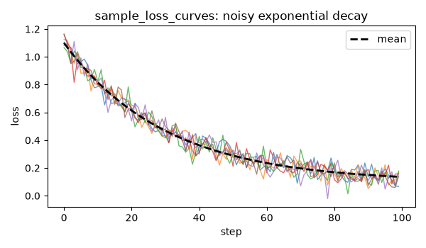
_images/sampler.png — Six curves from `sample_loss_curves` (independent steps) around the dashed mean curve. Both parts below reuse this exact sampler.¶

Part 1: catching regressions with the CLI¶

benchmarks/bench_synthetic.py samples one such curve per seed and reports min:loss at fixed checkpoints — exercising the list[dict] multi-step format and the min: lower-is-better convention. Two environment variables drive the walkthrough: PYBENCH_SYNTHETIC_REGRESS injects a regression (global lifts every checkpoint, local spikes the last), and PYBENCH_SYNTHETIC_RESAMPLE remaps each seed to a different curve so the re-run’s scores no longer match the baseline.

from synthetic import sample_loss_curves

_CHECKPOINTS = (1, 30, 100)


def bench_synthetic(seed: int, *, n_seeds: int = 30) -> list[dict]:
    if os.environ.get("PYBENCH_SYNTHETIC_RESAMPLE"):
        seed = int(np.random.default_rng(seed).integers(2**32))  # different curve
    rng = np.random.default_rng(seed)
    curve = sample_loss_curves(
        rng, n_seeds=1, n_steps=max(_CHECKPOINTS) + 1,
        amp=1.0, tau=30.0, floor=0.10, noise=0.05,
    )[0]
    losses = {s: float(curve[s]) for s in _CHECKPOINTS}
    regress = os.environ.get("PYBENCH_SYNTHETIC_REGRESS")
    if regress == "global":
        losses = {s: v + 0.05 for s, v in losses.items()}
    elif regress == "local":
        losses[_CHECKPOINTS[-1]] += 0.20
    return [{"step": s, "min:loss": losses[s]} for s in _CHECKPOINTS]

By default each seed reproduces its own curve exactly, so a clean re-run matches the baseline to the bit; the cases below add a regression — or resample the seeds — on top of that. The remap is deterministic, so every run is reproducible. Run the four cases in order.

First run — save the baseline. The first run has nothing to compare against; it samples 30 seeds, stores them, and marks the benchmark NEW.

$ uv run --package synthetic pybench examples/synthetic/benchmarks/
bench_synthetic   .......... NEW   1 metrics × 3 steps   (baseline saved)
──────────────────────────────────────────────────────────────
0 failed, 0 passed, 1 new  in 0.0s

Case 1 — no regression → PASS. Re-run unchanged. pybench reuses the stored seeds, every paired difference is zero, and nothing is flagged.

$ uv run --package synthetic pybench examples/synthetic/benchmarks/
bench_synthetic   .......... PASS   1 metrics × 3 steps   0/3 slots flagged
meta-p=1.000
──────────────────────────────────────────────────────────────
0 failed, 1 passed, 0 new  in 0.0s

Case 2 — resampled seeds, no regression → PASS. Set PYBENCH_SYNTHETIC_RESAMPLE=1: each seed now draws a different curve, so the current scores no longer equal the baseline’s. There is still no real regression, so the verdict stays PASS — proof that the verdict is a statistical test, not a score-equality check.

$ PYBENCH_SYNTHETIC_RESAMPLE=1 uv run --package synthetic pybench examples/synthetic/benchmarks/
bench_synthetic   .......... PASS   1 metrics × 3 steps   0/3 slots flagged
meta-p=1.000
──────────────────────────────────────────────────────────────
0 failed, 1 passed, 0 new  in 0.0s

Unlike Case 1, no two scores match — the curves were redrawn — yet none of the paired differences is large enough to flag, so pybench passes the noisy re-run.

Case 3 — global regression → FAIL. Lift every checkpoint. All three slots regress and the verdict flips.

$ PYBENCH_SYNTHETIC_REGRESS=global uv run --package synthetic pybench examples/synthetic/benchmarks/
bench_synthetic   .......... FAIL   1 metrics × 3 steps   3/3 slots flagged
meta-p=0.000
──────────────────────────────────────────────────────────────
1 failed, 0 passed, 0 new  in 0.0s

Case 4 — local regression → FAIL. Spike only the last checkpoint. A single flagged slot is enough; -v shows exactly which one:

$ PYBENCH_SYNTHETIC_REGRESS=local uv run --package synthetic pybench examples/synthetic/benchmarks/ -v
bench_synthetic   .......... FAIL   1 metrics × 3 steps   1/3 slots flagged
meta-p=0.000
  metric     step   baseline    current      Δ        p
  min:loss      1   1.08±0.05   1.08±0.05   +0.0%   1.000
  min:loss     30   0.46±0.04   0.46±0.04   +0.0%   1.000
  min:loss    100   0.13±0.06   0.33±0.06   -155.3%   0.000  ✗
──────────────────────────────────────────────────────────────
1 failed, 0 passed, 0 new  in 0.1s

That a single regressed checkpoint flips the verdict is the whole point — and the reason for the statistics in Part 2.

Part 2: why the severity permutation, rigorously¶

examples/synthetic/main.py revisits the no-regression, global, and local regimes as Monte-Carlo experiments and pits pybench’s verdict against the simpler tests it could have used. (The resampled Case 2 above is the single-shot version of the no-regression experiment here — over many replications it false-flags at exactly alpha.) It does not reimplement pybench’s statistics: the pybench verdict here calls the very functions the CLI runs — pybench.stats._severity and pybench.stats._sign_flip_meta_p, the within-seed sign-flip permutation of the continuous severity T = Σ max(0, t_crit − t_stat) (§3). Only the alternative tests, which are not part of pybench, are written out there:

a global t-test pooling every (seed, step) difference at once;
a per-step t-test + binomial on how many steps came out significant;
a sign-flip permutation on the flagged count (it respects the dependency between steps but throws away each slot’s magnitude);
the sign-flip permutation on the severity (pybench’s actual verdict, which keeps the magnitude).

uv run --package synthetic python examples/synthetic/main.py

The same exponential-decay sampler feeds all three cases; only the injected regression and the noise structure differ:

"""Doc plot: the two Part 2 data regimes (correlated null, localized spike)."""

import matplotlib.pyplot as plt
import numpy as np
from synthetic import sample_loss_curves

rng = np.random.default_rng(1)
kw = dict(amp=1.0, tau=30.0, floor=0.10, noise=0.05)

fig, (ax1, ax2) = plt.subplots(1, 2, figsize=(9, 3.2))
for row in sample_loss_curves(rng, n_seeds=6, n_steps=80, seed_sigma=0.05, **kw):
    ax1.plot(row, lw=1, alpha=0.8)
ax1.set(title="No-regression case: correlated steps", xlabel="step", ylabel="loss")

base = sample_loss_curves(rng, n_seeds=1, n_steps=60, **kw)[0]
cur = sample_loss_curves(rng, n_seeds=1, n_steps=60, **kw)[0]
cur[-1] += 0.33
ax2.plot(base, lw=1.5, label="baseline")
ax2.plot(cur, lw=1.5, label="regressed")
ax2.set(title="Local case: one regressed step", xlabel="step", ylabel="loss")
ax2.legend()
fig.tight_layout()

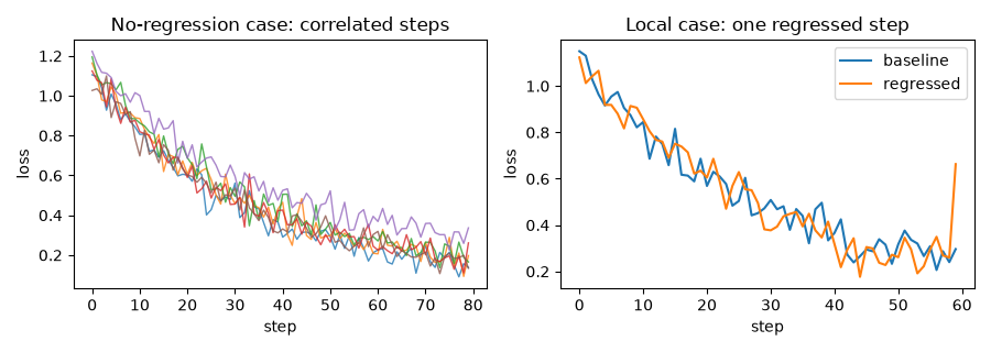
_images/regimes.png — Left, correlated curves (the no-regression case) — a per-seed offset shifts a whole curve, so the steps move together. Right, one regressed checkpoint (the local case) — a single step spikes while the rest match the baseline.¶

Each test’s false-positive rate (Case 1) and power (Cases 2 and 3), over 200 replications:

Case 1 — no regression, but the steps within a seed correlate
  test                              false-positive rate   (target = 0.05)
  global t-test (seed×step)                       0.405
  per-step t + binomial                           0.170
  sign-flip on count                              0.040
  sign-flip on severity (pybench)                 0.030

Case 2 — a global regression: every checkpoint's loss rises a little
  test                                   detection rate   (higher is better)
  global t-test (seed×step)                       1.000
  per-step t + binomial                           1.000
  sign-flip on count                              1.000
  sign-flip on severity (pybench)                 1.000

Case 3 — a local regression: one checkpoint spikes, the rest unchanged
  test                                   detection rate   (higher is better)
  global t-test (seed×step)                       0.225
  per-step t + binomial                           0.070
  sign-flip on count                              0.050
  sign-flip on severity (pybench)                 0.980

Case 1 — false alarms. With no real change, the global t-test pools correlated slots as independent (its standard error is too small) and the per-step binomial assumes the per-step rejections are independent (correlated steps reject together, over-dispersing the count) — they cry wolf 40% and 17% of the time. Both permutation tests stay at alpha: a permutation test is exactly calibrated whatever statistic it permutes.

Case 2 — the easy regression. When every checkpoint drifts together, all four tests catch it. This is the global t-test’s home turf, and pybench gives up no power here — its strengths in the other two cases cost it nothing on a broad regression.

Case 3 — missed regressions. A single checkpoint regresses sharply while the rest are unchanged. The global t-test dilutes that one spike across all 200 steps; the per-step binomial sees one significant step, indistinguishable from its alpha-rate false positives; and the sign-flip on count throws away the spike’s magnitude — one flag is one flag — so it misses too (5% detection, no better than chance). Only the sign-flip on severity, which keeps the spike’s magnitude, catches it (98%).

The lesson is twofold. Assuming the steps are independent (global t-test, per-step binomial) raises false alarms on correlated noise. And discarding effect magnitude (the count permutation) misses a regression hiding in a single slot. pybench’s permutation of the severity statistic does neither — which is exactly why §3.2 chose it. For the full walk-through of the machinery, see How it works.